This is adapted from the kaggle notebook here
https://
Imports
# Import libraries
import pandas as pd
import numpy as np

# For pre-processing and data sharing
from sklearn.model_selection import train_test_split

# For handling data imbalance
from imblearn.combine import SMOTETomek
from imblearn.under_sampling import TomekLinks

# To standardize the data
from sklearn.preprocessing import StandardScaler

# For feature selection
from sklearn.feature_selection import RFE

# Model machine learning
from sklearn.ensemble import RandomForestClassifier

# For model evaluation
from sklearn.metrics import accuracy_score, precision_score, recall_score, confusion_matrix
import seaborn as sns
import matplotlib.pyplot as plt


df = pd.read_csv('diabetes_binary_health_indicators_BRFSS2015.csv')
df.head()
Loading...
df.columnsIndex(['Diabetes_binary', 'HighBP', 'HighChol', 'CholCheck', 'BMI', 'Smoker',
'Stroke', 'HeartDiseaseorAttack', 'PhysActivity', 'Fruits', 'Veggies',
'HvyAlcoholConsump', 'AnyHealthcare', 'NoDocbcCost', 'GenHlth',
'MentHlth', 'PhysHlth', 'DiffWalk', 'Sex', 'Age', 'Education',
'Income'],
dtype='object')print(df.info())
print(df.describe())<class 'pandas.core.frame.DataFrame'>
RangeIndex: 253680 entries, 0 to 253679
Data columns (total 22 columns):
# Column Non-Null Count Dtype
--- ------ -------------- -----
0 Diabetes_binary 253680 non-null float64
1 HighBP 253680 non-null float64
2 HighChol 253680 non-null float64
3 CholCheck 253680 non-null float64
4 BMI 253680 non-null float64
5 Smoker 253680 non-null float64
6 Stroke 253680 non-null float64
7 HeartDiseaseorAttack 253680 non-null float64
8 PhysActivity 253680 non-null float64
9 Fruits 253680 non-null float64
10 Veggies 253680 non-null float64
11 HvyAlcoholConsump 253680 non-null float64
12 AnyHealthcare 253680 non-null float64
13 NoDocbcCost 253680 non-null float64
14 GenHlth 253680 non-null float64
15 MentHlth 253680 non-null float64
16 PhysHlth 253680 non-null float64
17 DiffWalk 253680 non-null float64
18 Sex 253680 non-null float64
19 Age 253680 non-null float64
20 Education 253680 non-null float64
21 Income 253680 non-null float64
dtypes: float64(22)
memory usage: 42.6 MB
None
Diabetes_binary HighBP HighChol CholCheck \
count 253680.000000 253680.000000 253680.000000 253680.000000
mean 0.139333 0.429001 0.424121 0.962670
std 0.346294 0.494934 0.494210 0.189571
min 0.000000 0.000000 0.000000 0.000000
25% 0.000000 0.000000 0.000000 1.000000
50% 0.000000 0.000000 0.000000 1.000000
75% 0.000000 1.000000 1.000000 1.000000
max 1.000000 1.000000 1.000000 1.000000
BMI Smoker Stroke HeartDiseaseorAttack \
count 253680.000000 253680.000000 253680.000000 253680.000000
mean 28.382364 0.443169 0.040571 0.094186
std 6.608694 0.496761 0.197294 0.292087
min 12.000000 0.000000 0.000000 0.000000
25% 24.000000 0.000000 0.000000 0.000000
50% 27.000000 0.000000 0.000000 0.000000
75% 31.000000 1.000000 0.000000 0.000000
max 98.000000 1.000000 1.000000 1.000000
PhysActivity Fruits ... AnyHealthcare NoDocbcCost \
count 253680.000000 253680.000000 ... 253680.000000 253680.000000
mean 0.756544 0.634256 ... 0.951053 0.084177
std 0.429169 0.481639 ... 0.215759 0.277654
min 0.000000 0.000000 ... 0.000000 0.000000
25% 1.000000 0.000000 ... 1.000000 0.000000
50% 1.000000 1.000000 ... 1.000000 0.000000
75% 1.000000 1.000000 ... 1.000000 0.000000
max 1.000000 1.000000 ... 1.000000 1.000000
GenHlth MentHlth PhysHlth DiffWalk \
count 253680.000000 253680.000000 253680.000000 253680.000000
mean 2.511392 3.184772 4.242081 0.168224
std 1.068477 7.412847 8.717951 0.374066
min 1.000000 0.000000 0.000000 0.000000
25% 2.000000 0.000000 0.000000 0.000000
50% 2.000000 0.000000 0.000000 0.000000
75% 3.000000 2.000000 3.000000 0.000000
max 5.000000 30.000000 30.000000 1.000000
Sex Age Education Income
count 253680.000000 253680.000000 253680.000000 253680.000000
mean 0.440342 8.032119 5.050434 6.053875
std 0.496429 3.054220 0.985774 2.071148
min 0.000000 1.000000 1.000000 1.000000
25% 0.000000 6.000000 4.000000 5.000000
50% 0.000000 8.000000 5.000000 7.000000
75% 1.000000 10.000000 6.000000 8.000000
max 1.000000 13.000000 6.000000 8.000000
[8 rows x 22 columns]
df['Diabetes_binary'].value_counts().plot(kind='pie')
df['Diabetes_binary'].value_counts()
Diabetes_binary
0.0 218334
1.0 35346
Name: count, dtype: int64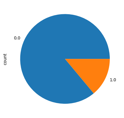
SPLIT DATA TRAIN & DATA TEST
# Separate features and targets
X = df.drop('Diabetes_binary', axis=1)
y = df['Diabetes_binary']

# Division of data into training data and test data
X_train, X_test, y_train, y_test = train_test_split(X, y, test_size=0.4)
Make sure the dataset is balanced
from imblearn.combine import SMOTETomek
# Split up the data
smt = SMOTETomek(tomek=TomekLinks(sampling_strategy='majority'))
X_train_resampled, y_train_resampled = smt.fit_resample(X_train, y_train)
# Resample
print('Class distribution before resampling:', np.bincount(y_train))
print('Class distribution before resampling:', np.bincount(y_train_resampled))
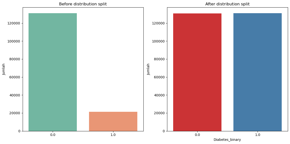
# Visualization of class distribution before and after
def plot_class_distribution(y_before, y_after, title_before, title_after):
fig, ax = plt.subplots(1, 2, figsize=(12, 6))
# Plot sebelum SMOTE-Tomek
sns.countplot(x=y_before, ax=ax[0], palette="Set2")
ax[0].set_title(title_before)
ax[0].set_xlabel("")
ax[0].set_ylabel("Jumlah")
# Plot sesudah SMOTE-Tomek
sns.countplot(x=y_after, ax=ax[1], palette="Set1")
ax[1].set_title(title_after)
ax[1].set_xlabel("Diabetes_binary")
ax[1].set_ylabel("Jumlah")
plt.tight_layout()
plt.show()
# Sebelum SMOTE-Tomek (y_train) dan Setelah SMOTE-Tomek (y_train_resampled)
plot_class_distribution(y_train, y_train_resampled, "Before distribution split", "After distribution split")/var/folders/bw/c9j8z20x45s2y20vv6528qjc0000gq/T/ipykernel_77798/1282855888.py:8: DeprecationWarning: Non-integer input passed to bincount. In a future version of NumPy, this will be an error. (Deprecated NumPy 2.1)
print('Class distribution before resampling:', np.bincount(y_train))
/var/folders/bw/c9j8z20x45s2y20vv6528qjc0000gq/T/ipykernel_77798/1282855888.py:9: DeprecationWarning: Non-integer input passed to bincount. In a future version of NumPy, this will be an error. (Deprecated NumPy 2.1)
print('Class distribution before resampling:', np.bincount(y_train_resampled))
/var/folders/bw/c9j8z20x45s2y20vv6528qjc0000gq/T/ipykernel_77798/1282855888.py:16: FutureWarning:
Passing `palette` without assigning `hue` is deprecated and will be removed in v0.14.0. Assign the `x` variable to `hue` and set `legend=False` for the same effect.
sns.countplot(x=y_before, ax=ax[0], palette="Set2")
Class distribution before resampling: [130931  21277]
Class distribution before resampling: [130840 130931]
/var/folders/bw/c9j8z20x45s2y20vv6528qjc0000gq/T/ipykernel_77798/1282855888.py:22: FutureWarning:

Passing `palette` without assigning `hue` is deprecated and will be removed in v0.14.0. Assign the `x` variable to `hue` and set `legend=False` for the same effect.

  sns.countplot(x=y_after, ax=ax[1], palette="Set1")
Feature Selection
from sklearn.feature_selection import RFECV

# The "accuracy" scoring is proportional to the number of correct classifications
estimator2= RandomForestClassifier()
rfecv = RFECV(estimator=estimator2, step=1, n_jobs=-1, cv=5, scoring='recall')   #5-fold cross-validation
rfecv = rfecv.fit(X_train_resampled, y_train_resampled)

# Get the best features selected by RFE
selected_rfecv = X_train_resampled.columns[rfecv.support_]

print('Optimal number of features :', rfecv.n_features_)
print('Best features :', selected_rfecv)
Optimal number of features : 18
Best features : Index(['HighBP', 'HighChol', 'BMI', 'Smoker', 'HeartDiseaseorAttack',
'PhysActivity', 'Fruits', 'Veggies', 'HvyAlcoholConsump', 'NoDocbcCost',
'GenHlth', 'MentHlth', 'PhysHlth', 'DiffWalk', 'Sex', 'Age',
'Education', 'Income'],
dtype='object')
# Create a new DataFrame with only the selected features
X_train_selected_rfecv = X_train_resampled[selected_rfecv]
X_test_selected_rfecv = X_test[selected_rfecv]
Random Forest
# Initialize the Random Forest
rf_model = RandomForestClassifier(bootstrap= True,
n_estimators=200, n_jobs=-1,
max_depth=20, max_features='sqrt',
min_samples_leaf=1,
max_leaf_nodes = 150,
min_samples_split = 5,
random_state=42)
# Train the model on the processed training data
rf_model.fit(X_train_selected_rfecv, y_train_resampled)
# Prediction on test data
y_pred = rf_model.predict(X_test_selected_rfecv)
# Evaluate model performance
accuracy = accuracy_score(y_test, y_pred)
precision = precision_score(y_test, y_pred)
recall = recall_score(y_test, y_pred)
print("Accuracy: {:.2f}%".format(accuracy * 100))
print("Precision: {:.2f}%".format(precision * 100))
print("Recall: {:.2f}%".format(recall * 100))
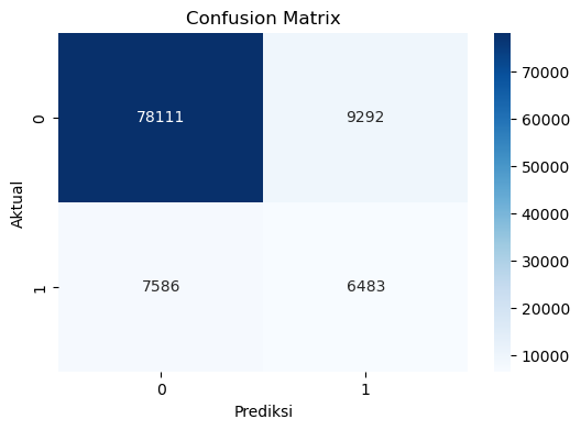
# Confusion Matrix
cf_matrix = confusion_matrix(y_test, y_pred)
# Plot Confusion Matrix
plt.figure(figsize=(6,4))
sns.heatmap(cf_matrix, annot=True, fmt='d', cmap='Blues')
plt.xlabel('Prediksi')
plt.ylabel('Aktual')
plt.title('Confusion Matrix')
plt.show()Accuracy: 83.37%
Precision: 41.10%
Recall: 46.08%
# Evaluate model performance on training data
y_train_pred = rf_model.predict(X_train_selected_rfecv)
train_accuracy = accuracy_score(y_train_resampled, y_train_pred)
print("Training Accuracy: {:.2f}%".format(train_accuracy * 100))

# Evaluate model performance on test data
test_accuracy = accuracy_score(y_test, y_pred)
print("Test Accuracy: {:.2f}%".format(test_accuracy * 100))
Training Accuracy: 87.63%
Test Accuracy: 83.37%
KNN
# Model machine learning
from sklearn.neighbors import KNeighborsClassifier
# Initialize KNN model
knn_model = KNeighborsClassifier(n_neighbors=5, weights='uniform', algorithm='auto', n_jobs=-1)
# Train the model on pre-processed training data
knn_model.fit(X_train_selected_rfecv, y_train_resampled)
# Prediction on test data
y_pred_knn = knn_model.predict(X_test_selected_rfecv)
# Evaluate model performance
accuracy_knn = accuracy_score(y_test, y_pred_knn)
precision_knn = precision_score(y_test, y_pred_knn)
recall_knn = recall_score(y_test, y_pred_knn)
print("Accuracy: {:.2f}%".format(accuracy_knn * 100))
print("Precision: {:.2f}%".format(precision_knn * 100))
print("Recall: {:.2f}%".format(recall_knn * 100))
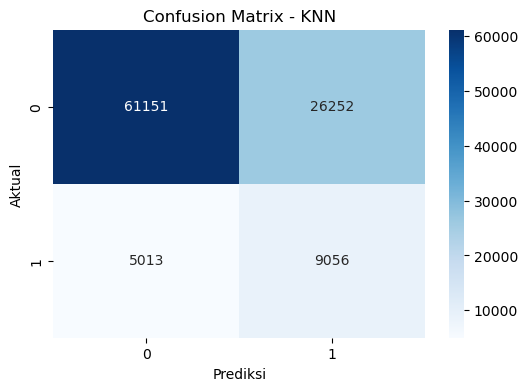
# Confusion Matrix
cf_matrix_knn = confusion_matrix(y_test, y_pred_knn)
# Plot Confusion Matrix
plt.figure(figsize=(6,4))
sns.heatmap(cf_matrix_knn, annot=True, fmt='d', cmap='Blues')
plt.xlabel('Prediksi')
plt.ylabel('Aktual')
plt.title('Confusion Matrix - KNN')
plt.show()Accuracy: 69.19%
Precision: 25.65%
Recall: 64.37%
# Evaluate model performance on training data
y_train_pred_knn = knn_model.predict(X_train_selected_rfecv)
train_accuracy_knn = accuracy_score(y_train_resampled, y_train_pred_knn)
print("Training Accuracy: {:.2f}%".format(train_accuracy_knn * 100))

# Evaluate model performance on the test data
test_accuracy_knn = accuracy_score(y_test, y_pred_knn)
print("Test Accuracy: {:.2f}%".format(test_accuracy_knn * 100))
Training Accuracy: 88.19%
Test Accuracy: 69.19%
SVM
from sklearn.svm import SVC

# Initialize SVM model
svm_model = SVC(kernel='rbf', C=1, gamma='scale', random_state=42)

# Train the model on pre-processed training data (diabetes risk classification)
svm_model.fit(X_train_selected_rfecv, y_train_resampled)

# Prediction on test data using SVM
y_pred_svm = svm_model.predict(X_test_selected_rfecv)

# Evaluation of SVM model performance
accuracy_svm = accuracy_score(y_test, y_pred_svm)
precision_svm = precision_score(y_test, y_pred_svm, pos_label=1)
recall_svm = recall_score(y_test, y_pred_svm, pos_label=1)

print("=== SVM untuk Klasifikasi Risiko Diabetes ===")
print("Accuracy: {:.2f}%".format(accuracy_svm * 100))
print("Precision: {:.2f}%".format(precision_svm * 100))
print("Recall: {:.2f}%".format(recall_svm * 100))

# Confusion Matrix for SVM model
cf_matrix_svm = confusion_matrix(y_test, y_pred_svm)

# Plot Confusion Matrix for SVM model
plt.figure(figsize=(6, 4))
sns.heatmap(cf_matrix_svm, annot=True, fmt='d', cmap='Blues')
plt.xlabel('Prediksi')
plt.ylabel('Aktual')
plt.title('Confusion Matrix - SVM (Klasifikasi Risiko Diabetes)')
plt.show()
# Evaluate model performance on training data
y_train_pred_svm = svm_model.predict(X_train_selected_rfecv)
train_accuracy_svm = accuracy_score(y_train_resampled, y_train_pred_svm)
print("Training Accuracy: {:.2f}%".format(train_accuracy_svm * 100))
# Evaluate model performance on test data
test_accuracy_svm = accuracy_score(y_test, y_pred)
print("Test Accuracy: {:.2f}%".format(test_accuracy_svm * 100))import matplotlib.pyplot as plt
import numpy as np
from sklearn.metrics import accuracy_score, precision_score, recall_score, f1_score, roc_auc_score
# Prediksi dengan model
y_pred_knn_model = knn_model.predict(X_test_selected_rfecv)
y_pred_rf_model = rf_model.predict(X_test_selected_rfecv)
y_pred_svm_model = svm_model.predict(X_test_selected_rfecv)
# Evaluasi metrik untuk masing-masing model
models = ['KNN', 'Random Forest', 'SVM']
accuracy = [
accuracy_score(y_test, y_pred_knn_model),
accuracy_score(y_test, y_pred_rf_model),
accuracy_score(y_test, y_pred_svm_model)
]
precision = [
precision_score(y_test, y_pred_knn_model),
precision_score(y_test, y_pred_rf_model),
precision_score(y_test, y_pred_svm_model)
]
recall = [
recall_score(y_test, y_pred_knn_model),
recall_score(y_test, y_pred_rf_model),
recall_score(y_test, y_pred_svm_model)
]
f1 = [
f1_score(y_test, y_pred_knn_model),
f1_score(y_test, y_pred_rf_model),
f1_score(y_test, y_pred_svm_model)
]
roc_auc = [
roc_auc_score(y_test, y_pred_knn_model),
roc_auc_score(y_test, y_pred_rf_model),
roc_auc_score(y_test, y_pred_svm_model)
]
# Data untuk visualisasi
metrics = ['Accuracy', 'Precision', 'Recall', 'F1-Score', 'ROC-AUC']
values = [accuracy, precision, recall, f1, roc_auc]
# Plot hasil perbandingan dalam bentuk bar plot
fig, axes = plt.subplots(1, len(metrics), figsize=(20, 5))
for i, metric in enumerate(metrics):
axes[i].bar(models, values[i], color=['blue', 'red','green'])
axes[i].set_title(metric)
axes[i].set_ylim([0, 1])
axes[i].set_ylabel('Score')
for j, val in enumerate(values[i]):
axes[i].text(j, val + 0.02, f'{val:.2f}', ha='center', va='bottom')
plt.tight_layout()
plt.show()