Import Libraries and Install Dependencies
import pandas as pd
import numpy as np
from sklearn.preprocessing import StandardScaler
from sklearn.cluster import KMeans
import matplotlib.pyplot as plt
import seaborn as sns

# Set random seed for reproducibility
np.random.seed(42)
Load Data
# Read the TSV file
df = pd.read_csv('Filtered_Diff_Exp.tsv', sep='\t')

# Let's look at the first few rows and basic information about our dataset
print("First few rows of the dataset:")
print(df.head())
print("\nDataset information:")
print(df.info())
First few rows of the dataset:
feature_ids Ath_WT_R1_expression Ath_WT_R2_expression \
0 AT3G14770 5.019769 4.945506
1 AT4G12460 1.152617 0.409854
2 AT1G68790 1.172865 1.135914
3 AT5G16780 1.133932 0.777333
4 AT3G05130 1.702084 1.425840
Ath_hy5_R1_expression Ath_hy5_R2_expression
0 3.050257 3.115209
1 2.701273 2.982812
2 3.096043 3.458751
3 3.527632 4.079876
4 3.871323 3.896601
Dataset information:
<class 'pandas.core.frame.DataFrame'>
RangeIndex: 612 entries, 0 to 611
Data columns (total 5 columns):
# Column Non-Null Count Dtype
--- ------ -------------- -----
0 feature_ids 612 non-null object
1 Ath_WT_R1_expression 612 non-null float64
2 Ath_WT_R2_expression 612 non-null float64
3 Ath_hy5_R1_expression 612 non-null float64
4 Ath_hy5_R2_expression 612 non-null float64
dtypes: float64(4), object(1)
memory usage: 24.0+ KB
None
Clustering Analysis
# Calculate mean expression for wild type (WT) and hy5 mutant
df['WT_mean'] = df[['Ath_WT_R1_expression', 'Ath_WT_R2_expression']].mean(axis=1)
df['hy5_mean'] = df[['Ath_hy5_R1_expression', 'Ath_hy5_R2_expression']].mean(axis=1)

# Create a new dataframe with just the mean values
expression_data = df[['feature_ids', 'WT_mean', 'hy5_mean']]

print("First few rows with mean expression values:")
print(expression_data.head())
First few rows with mean expression values:
feature_ids WT_mean hy5_mean
0 AT3G14770 4.982637 3.082733
1 AT4G12460 0.781235 2.842043
2 AT1G68790 1.154389 3.277397
3 AT5G16780 0.955633 3.803754
4 AT3G05130 1.563962 3.883962
Raw Expression Data:
- Each row shows a unique Arabidopsis gene (e.g., AT3G14770)
- WT_mean shows average expression in normal plants
- hy5_mean shows average expression in the mutant
- Looking at AT3G14770: expression decreases in mutant (4.98 → 3.08)
- Looking at AT4G12460: expression increases in mutant (0.78 → 2.84)
# Extract features for clustering (excluding gene IDs)
X = expression_data[['WT_mean', 'hy5_mean']].values

# Scale the data
scaler = StandardScaler()
X_scaled = scaler.fit_transform(X)

print("Shape of scaled data:", X_scaled.shape)
print("\nFirst few rows of scaled data:")
print(X_scaled[:5])
Shape of scaled data: (612, 2)
First few rows of scaled data:
[[ 1.04312184 -0.35210941]
[-0.69262915 -0.48487966]
[-0.53846578 -0.24472823]
[-0.62057917 0.04562283]
[-0.36925646 0.08986728]]
Scaled Data:
- Shape (612, 2) means we have 612 genes with 2 measurements each
- Data has been standardized (centered and scaled) for clustering
- Values are now in standard deviations from the mean
- Positive values = above average expression
- Negative values = below average expression
- Example: First gene has above-average WT expression (1.04) but below-average hy5 expression (-0.35)
The scaling step is crucial because it puts all measurements on the same scale, making the clustering analysis more reliable and interpretable.
# Calculate inertia for different numbers of clusters
inertias = []
K = range(1, 11)

for k in K:
    kmeans = KMeans(n_clusters=k, random_state=42)
    kmeans.fit(X_scaled)
    inertias.append(kmeans.inertia_)

# Plot elbow curve
plt.figure(figsize=(10, 6))
plt.plot(K, inertias, 'bx-')
plt.xlabel('k')
plt.ylabel('Inertia')
plt.title('Elbow Method For Optimal k')
plt.grid(True)
plt.show()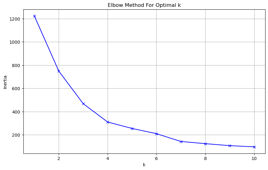
The elbow method plot shows how the inertia (within-cluster sum of squares) changes as we increase the number of clusters (k). Think of inertia as a measure of how spread out the data points are within their assigned clusters - lower inertia means the clusters are more compact and well-defined. In this plot, we can see a sharp bend (the “elbow”) around k=3 or k=4. This bend is significant because:
Before the elbow (k=1 to k=3), adding more clusters dramatically reduces the inertia. This tells us that each additional cluster is providing a substantial improvement in explaining the data’s structure. After the elbow (k>4), the line starts to flatten out. Adding more clusters yields diminishing returns - we’re not getting as much benefit from splitting the data further.
Based on this visualization, I would recommend using k=4 clusters for our analysis. Here’s why:
It’s right at the elbow point where we get good cluster separation The inertia has stabilized enough to suggest we’ve captured the main patterns With 4 clusters, we’ll likely be able to interpret meaningful biological differences between groups of genes
# Create a copy of the data first
kmeans = KMeans(n_clusters=4, random_state=42)
clusters = kmeans.fit_predict(X_scaled)
expression_data = expression_data.copy()
expression_data['Cluster'] = clusters
print("Number of genes in each cluster:")
print(expression_data['Cluster'].value_counts())
Number of genes in each cluster:
Cluster
0 295
1 177
2 105
3 35
Name: count, dtype: int64
# Create scatter plot
plt.figure(figsize=(12, 8))
scatter = plt.scatter(expression_data['WT_mean'],
                     expression_data['hy5_mean'],
                     c=expression_data['Cluster'],
                     cmap='viridis')
plt.xlabel('Wild Type Expression (mean)')
plt.ylabel('hy5 Mutant Expression (mean)')
plt.title('Gene Expression Clusters')
plt.colorbar(scatter, label='Cluster')

# Add a diagonal line for reference
min_val = min(expression_data['WT_mean'].min(), expression_data['hy5_mean'].min())
max_val = max(expression_data['WT_mean'].max(), expression_data['hy5_mean'].max())
plt.plot([min_val, max_val], [min_val, max_val], 'r--', alpha=0.5)

plt.grid(True, alpha=0.3)
plt.show()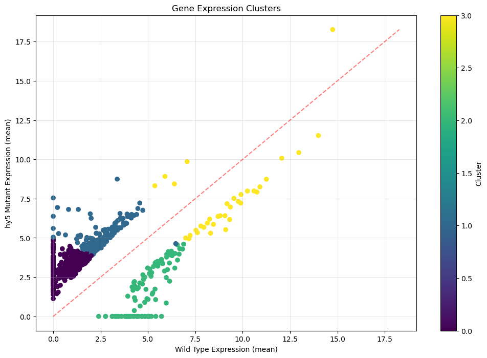
Looking at this scatter plot of gene expression data, here are the key observations:
Cluster 0 (Purple dots, bottom left):
- Concentrated in low Wild Type expression (0-2.5 on x-axis)
- Shows higher expression in hy5 mutant (2-5 on y-axis)
- Forms a dense cluster above the diagonal red line, indicating consistent upregulation
Cluster 1 (Blue dots, middle):
- Moderate Wild Type expression (2-5 on x-axis)
- Consistently higher expression in hy5 mutant (4-7 on y-axis)
- Sits distinctly above the diagonal, showing clear upregulation
Cluster 2 (Green dots, middle-right):
- Strong Wild Type expression (5-7.5 on x-axis)
- Lower expression in hy5 mutant (0-4 on y-axis)
- Falls below the diagonal line, indicating downregulation
Cluster 3 (Yellow dots, top right):
- Highest Wild Type expression (7.5-15 on x-axis)
- Maintains high expression in mutant (5-18 on y-axis)
- Clusters near the diagonal line, suggesting minimal change
def calculate_cluster_patterns(df, fold_change_threshold=1.5):
    """
    Analyze gene expression patterns for each cluster, providing comprehensive statistics
    about how genes respond to the absence of HY5.

    Args:
        df: DataFrame containing gene expression data with WT_mean and hy5_mean columns
        fold_change_threshold: Minimum fold change to consider a gene significantly regulated

    Returns:
        Three DataFrames containing basic statistics, expression ratios, and regulation patterns
    """
    # Calculate basic statistics for each cluster
    # We separate WT and hy5 calculations for clarity
    wt_stats = df.groupby('Cluster')['WT_mean'].agg(['mean', 'std', 'count']).round(2)
    hy5_stats = df.groupby('Cluster')['hy5_mean'].agg(['mean', 'std']).round(2)

    # Combine statistics into a multi-level column DataFrame
    cluster_stats = pd.concat({
        'WT_mean': wt_stats,
        'hy5_mean': hy5_stats
    }, axis=1)

    # Calculate expression ratios with careful handling of low expression values
    def calculate_stable_ratio(group):
        """
        Calculate expression ratios while avoiding division by very small numbers.
        Only considers genes with meaningful WT expression (>0.1) to prevent inflated ratios.
        """
        meaningful_expression = group['WT_mean'] > 0.1
        if meaningful_expression.any():
            ratios = group[meaningful_expression]['hy5_mean'] / group[meaningful_expression]['WT_mean']
            return ratios.mean()
        return 0  # Return 0 if no genes meet the criteria

    # Calculate ratios using our stable method
    ratios = df.groupby('Cluster').apply(
        calculate_stable_ratio,
        include_groups=False
    ).round(2)

    # Calculate the percentage of genes showing significant regulation
    patterns = pd.DataFrame({
        'Upregulated in hy5': df.groupby('Cluster').apply(
            lambda x: (x['hy5_mean'] > x['WT_mean'] * fold_change_threshold).mean() * 100,
            include_groups=False
        ),
        'Downregulated in hy5': df.groupby('Cluster').apply(
            lambda x: (x['hy5_mean'] < x['WT_mean'] / fold_change_threshold).mean() * 100,
            include_groups=False
        )
    }).round(1)

    return cluster_stats, ratios, patterns

# Calculate all statistics
cluster_stats, cluster_ratios, regulation_patterns = calculate_cluster_patterns(expression_data)

# Print results with informative headers
print("Cluster Statistics:")
print("This shows the mean expression, standard deviation, and number of genes in each cluster")
print(cluster_stats)
print("\nAverage hy5/WT expression ratio for each cluster:")
print("(Ratios calculated only for genes with meaningful WT expression)")
print(cluster_ratios)
print("\nRegulation patterns (percentage of genes):")
print("(Shows what fraction of genes are significantly up- or down-regulated)")
print(regulation_patterns)
Cluster Statistics:
This shows the mean expression, standard deviation, and number of genes in each cluster
WT_mean hy5_mean
mean std count mean std
Cluster
0 0.77 0.64 295 3.18 0.68
1 2.46 0.90 177 5.03 0.83
2 4.96 0.99 105 1.77 1.58
3 9.15 2.13 35 7.49 2.51
Average hy5/WT expression ratio for each cluster:
(Ratios calculated only for genes with meaningful WT expression)
Cluster
0 3.85
1 2.39
2 0.32
3 0.83
dtype: float64
Regulation patterns (percentage of genes):
(Shows what fraction of genes are significantly up- or down-regulated)
Upregulated in hy5 Downregulated in hy5
Cluster
0 100.0 0.0
1 98.3 0.0
2 0.0 97.1
3 5.7 8.6
Here’s a concise summary of the HY5 gene expression clusters in bullet points:
Cluster 0 (295 genes) - Strong Repression:
- Very low expression with HY5 (0.77), jumps to 3.18 without HY5
- 100% of genes show upregulation in mutant
- HY5 acts as a strong repressor for these genes
Cluster 1 (177 genes) - Moderate Repression:
- Moderate expression with HY5 (2.46), increases to 5.03 without HY5
- 98.3% show upregulation in mutant
- Maintains some baseline expression even with HY5 present
Cluster 2 (105 genes) - HY5-Dependent Activation:
- Strong expression with HY5 (4.96), drops to 1.77 without HY5
- 97.1% show downregulation in mutant
- HY5 acts as an activator for these genes
Cluster 3 (35 genes) - HY5-Independent:
- High expression in both conditions (9.15 → 7.49)
- Minimal regulation by HY5 (only 5.7% up, 8.6% down)
- Likely controlled by other regulatory factors
Key takeaway: HY5 can act as either a repressor or activator depending on the target genes, with some genes being largely independent of its control.